flowchart LR
  A[SIPSA / DANE<br/>monthly prices] --> B[COP → USD<br/>quantmod rates]
  B --> C[Spline interpolation<br/>of gaps]
  C --> D[ts object<br/>freq = 12]
  D --> E[Decomposition<br/>trend + season]
  D --> F[ADF tests<br/>differencing]
  F --> G{Train 2012–2023<br/>Test 2024–2025}
  G --> H[auto.arima]
  G --> I[Manual ARIMA]
  G --> J[SARIMA]
  G --> K[ARIMA-GARCH]
  H & I & J & K --> L[Diagnostics<br/>Ljung-Box · normality · ARCH]
  L --> M[Test RMSE / MAE / MAPE<br/>+ interactive plots]
Tahiti lemon price forecasting in Colombia
Time series
Forecasting
Agricultural economics
R
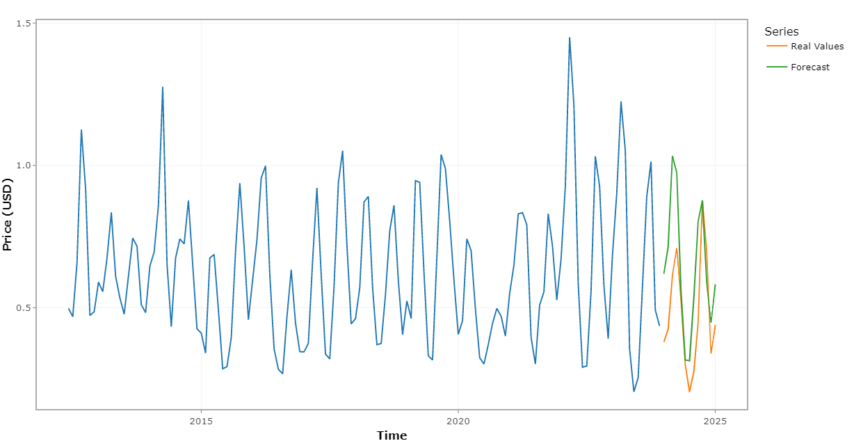
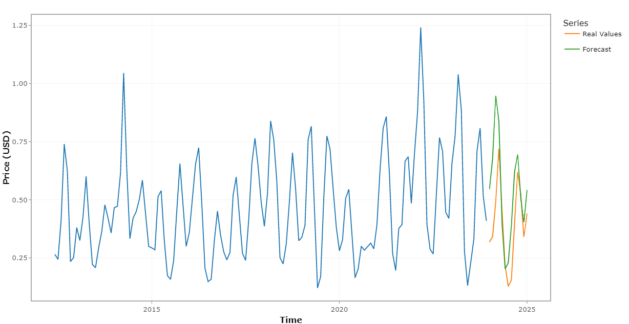
Time-series analysis and SARIMA forecasts of monthly wholesale lemon prices in Bogotá, Medellín and Bucaramanga (2012–2025), with interactive forecast plots.
3 largest wholesale markets in Colombia
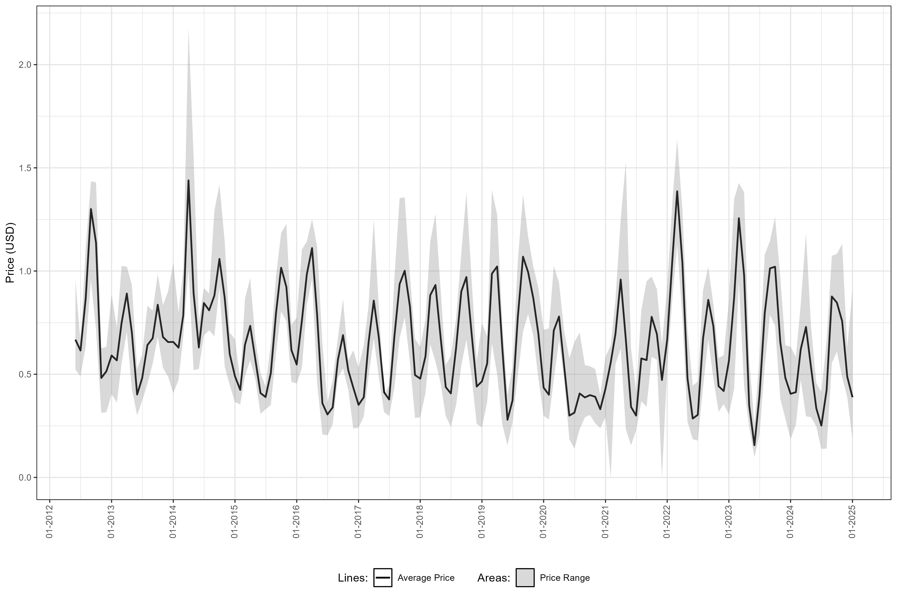
2012–2025 monthly prices from SIPSA / DANE
4 models auto ARIMA, ARIMA, SARIMA, ARIMA-GARCH
13 months held-out test set (2024–Jan 2025)
The problem
Tahiti lemon (Citrus latifolia) prices in Colombia swing with the harvest season. Farmers decide when to sell and traders decide when to buy, so both need to know when prices peak and what to expect in the coming months. This was the final project of my MBA in Data Science and Analytics (USP).
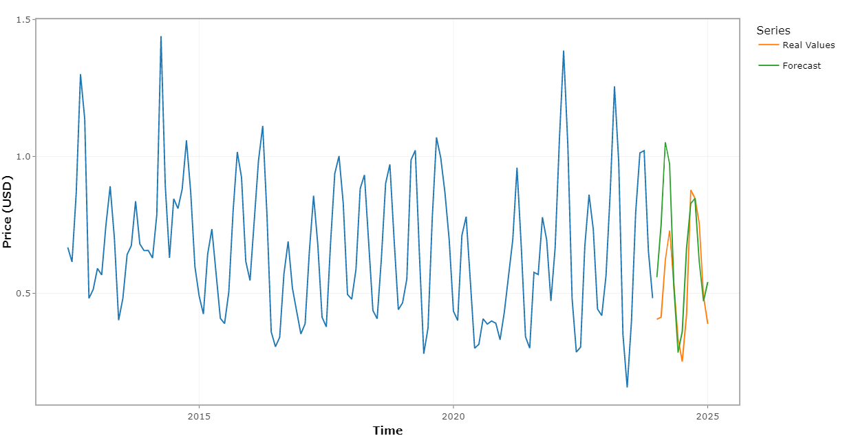
Interactive forecasts
Zoom, hover and toggle series in the plots below (built with plotly in R).
Pipeline architecture
Theory
1. Decomposition
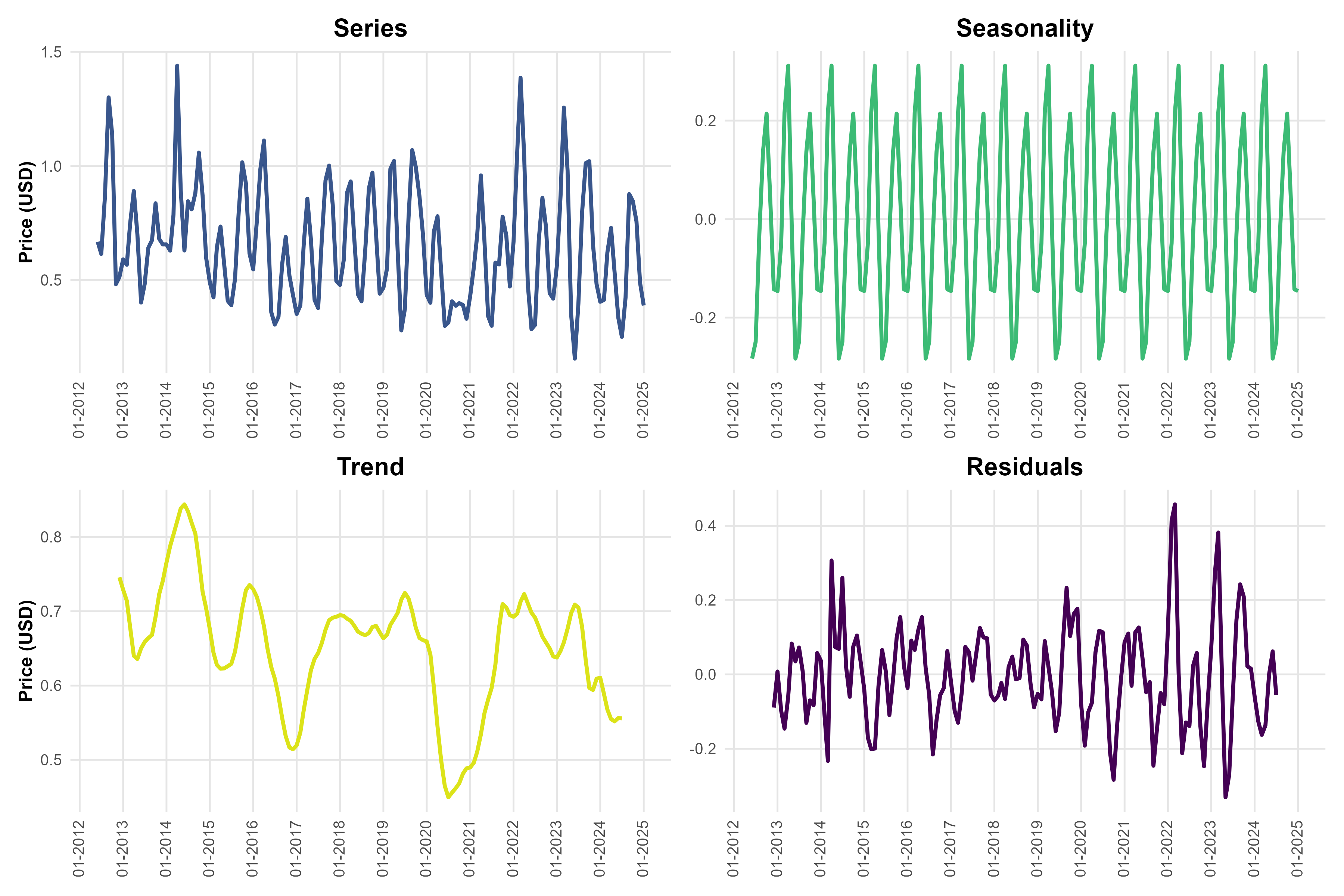
A monthly price series is split into trend \(T_t\), seasonality \(S_t\) and remainder \(R_t\), additively or multiplicatively (when seasonal swings grow with the price level):
\[ y_t = T_t + S_t + R_t \qquad\text{or}\qquad y_t = T_t \times S_t \times R_t . \]
2. Stationarity: Augmented Dickey-Fuller test
ARIMA models need a stationary series. The ADF regression tests for a unit root (\(H_0: \gamma = 0\), non-stationary):
\[ \Delta y_t = \alpha + \beta t + \gamma\, y_{t-1} + \sum_{i=1}^{p}\delta_i\,\Delta y_{t-i} + \varepsilon_t . \]
If \(H_0\) is not rejected, the series is differenced (\(\Delta y_t = y_t - y_{t-1}\)) and tested again.
3. Seasonal ARIMA
With the backshift operator \(B y_t = y_{t-1}\) and season length \(s = 12\), a SARIMA\((p,d,q)(P,D,Q)_{12}\) model is
\[ \Phi_P(B^{s})\,\phi_p(B)\,(1-B)^{d}(1-B^{s})^{D}\,y_t \;=\; \Theta_Q(B^{s})\,\theta_q(B)\,\varepsilon_t, \qquad \varepsilon_t \sim WN(0,\sigma^2), \]
where \(\phi_p, \theta_q\) are the short-term AR and MA polynomials and \(\Phi_P, \Theta_Q\) their seasonal counterparts. The models compared were selected by auto.arima (AICc search), ARIMA\((1,0,1)(0,1,1)_{12}\) and SARIMA\((2,1,1)(2,1,1)_{12}\).
4. Residual diagnostics
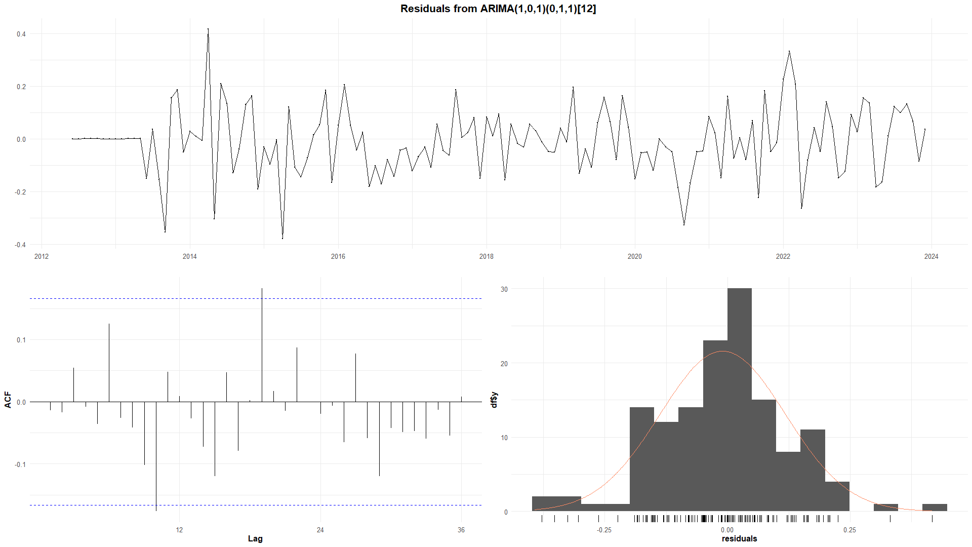
A good model leaves white-noise residuals. The Ljung-Box statistic tests for leftover autocorrelation up to lag \(h\):
\[ Q = n(n+2)\sum_{k=1}^{h}\frac{\hat\rho_k^{2}}{n-k} \;\sim\; \chi^2_{h-m}. \]
The ARCH LM test checks whether the residual variance changes over time. If it does, a GARCH(1,1) models the conditional variance:
\[ \sigma_t^{2} = \omega + \alpha\,\varepsilon_{t-1}^{2} + \beta\,\sigma_{t-1}^{2}. \]
5. Forecast accuracy on the test set
\[ \text{RMSE} = \sqrt{\tfrac{1}{h}\textstyle\sum_t (y_t-\hat y_t)^2},\qquad \text{MAE} = \tfrac{1}{h}\textstyle\sum_t |y_t-\hat y_t|,\qquad \text{MAPE} = \tfrac{100}{h}\textstyle\sum_t \left|\tfrac{y_t-\hat y_t}{y_t}\right| . \]
From the equations to R
Condensed from 01_Serie_Bogota_ENG.R. Hover over the numbers to link each line to the theory above.
prices_ts <- ts(complete_data[, 8], start = c(2012, 6),
end = c(2025, 1), frequency = 12)
decompose(prices_ts, type = "multiplicative")
price_train <- window(prices_ts, start = c(2012, 6), end = c(2023, 12))
price_test <- window(prices_ts, start = c(2024, 1), end = c(2025, 1))
adf.test(prices_ts, alternative = "stationary")
adf.test(diff(prices_ts))
arima_auto <- auto.arima(price_train, trace = TRUE)
sarima <- Arima(price_train, order = c(2, 1, 1),
seasonal = c(2, 1, 1))
checkresiduals(sarima)
ArchTest(residuals(sarima))
fc <- forecast(sarima, h = length(price_test))
accuracy(fc, price_test)
spec <- ugarchspec(variance.model = list(model = "sGARCH", garchOrder = c(1, 1)),
mean.model = list(armaOrder = c(2, 1)))
garch <- ugarchfit(spec, data = price_train)- 1
- Monthly series (\(s = 12\)) of average prices in USD, after spline interpolation of missing months.
- 2
- Decomposition \(y_t = T_t \times S_t \times R_t\).
- 3
- Train 2012–2023, test 2024–Jan 2025: the forecast is judged on months the model never saw.
- 4
- ADF unit-root test on the series and on its first difference.
- 5
- Automatic order search by AICc.
- 6
- SARIMA\((2,1,1)(2,1,1)_{12}\): seasonal and non-seasonal differencing plus AR/MA terms.
- 7
- Ljung-Box test and residual ACF/histogram.
- 8
- ARCH LM test for changing variance.
- 9
- Test-set RMSE, MAE and MAPE.
- 10
- GARCH(1,1) for the conditional variance \(\sigma_t^2 = \omega + \alpha\varepsilon_{t-1}^2 + \beta\sigma_{t-1}^2\).
Figures
Skills shown: time-series modelling and diagnostics, forecasting and out-of-sample evaluation, volatility models, public economic data, interactive visualization (plotly), R (forecast, tseries, urca, rugarch, fpp3).