flowchart LR
  A[Raw Nordic barley<br/>VCU trials 2014–2024] --> B[Stage I<br/>pairwise MI audit]
  B --> C[Chance correction<br/>by permutation]
  C --> D[Pure-linear null<br/>excess information]
  B --> E[Stage II<br/>predictive validation]
  E --> F[Stage IIIA<br/>FA readiness audit]
  F --> G[Stage IIIB<br/>reduced-rank FA models]
  G --> H[Stage IIIC<br/>MI on FA residuals]
  H --> I[Stage IIID<br/>entropy + spatial classes]
Beyond linear G×E in Nordic barley
G×E
Mixed models
Information theory
Reproducible research
R
Factor-analytic mixed models plus mutual information and entropy on 26,000 observations from Nordic spring-barley trials. A publication-grade, fully reproducible research package.
Code on GitHub Methods document Results document
26,028 observations · 471 cultivars · 762 environments
92.75% of the cultivar × environment matrix is empty
0.31 vs 0.09 median residual NMI vs matched linear null
98.5% of selected pairs carry information beyond linear
The question
Genotype-by-environment interaction (G×E) decides which cultivar to recommend where. Factor-analytic (FA) mixed models are the standard tool: they summarize how cultivars respond across many environments with a few latent factors. But FA is linear and low-rank. How much dependence between environments is left after FA, is it non-linear, and where is it?
The idea of this project is to treat FA modelling and information theory as complementary layers: FA captures the dominant linear structure, and mutual information plus entropy diagnose what remains.
Pipeline architecture
Each stage lives in its own folder (analysis/stage_0X_.../) with a README, canonical code and results, so any figure can be traced back to the script that made it.
Theory
1. Relative performance within environment
National trial systems differ in yield level, so yield is standardized inside each environment \(e\) for cultivar \(g\):
\[ z_{ge} = \frac{y_{ge} - \bar y_e}{s_e}. \]
2. Mutual information between environments
For two environments sharing enough cultivars, their standardized profiles are discretized into equal-frequency bins (3 in the main analysis) and compared with
\[ MI(X,Y) = \sum_{x,y} p(x,y)\,\log\frac{p(x,y)}{p(x)\,p(y)}, \qquad NMI(X,Y) = \frac{MI(X,Y)}{\sqrt{H(X)\,H(Y)}} . \]
3. Correcting the finite-sample bias
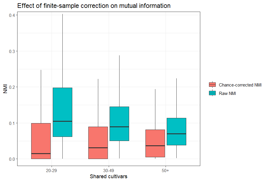
Raw NMI is biased upwards when few cultivars are shared. One profile is permuted \(B = 199\) times, keeping sample size and marginal distributions fixed, and the chance level is subtracted:
\[ cNMI = \max\left\{0,\ NMI_{obs} - \overline{NMI}_{perm}\right\}. \]
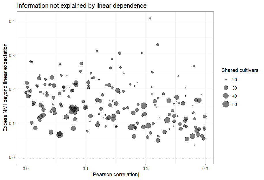
4. Is it more than correlation? The pure-linear null
For pairs with weak Pearson correlation but high cNMI, simulated data keep the same Pearson correlation but are otherwise linear. The excess information is
\[ eNMI = NMI_{obs} - \mathbb E\left[NMI_{\text{linear null}}\right]. \]
5. Reduced-rank factor-analytic model
After completing the sparse environment × cultivar matrix (nuclear-norm regularization with softImpute) and an SVD for the initial cultivar loadings, FA models of order \(k = 1, 2, 3\) are fitted with lme4:
\[ z_{ge} = \alpha_g + \sum_{h=1}^{k} \lambda_{gh}\, w_{eh} + \varepsilon_{ge}, \]
where \(\alpha_g\) is the cultivar mean (fixed), \(\lambda_{gh}\) are the loadings from the SVD and \(w_{eh}\) are random environmental scores.
NotePrecise about what this is
This is a two-stage reduced-rank / PC-FA model, not a single joint REML fit of a general FA covariance. And the sign of an FA axis is arbitrary: flipping both loadings and scores gives the same fit, so maps are read by relative position and magnitude.
6. What FA removes, and how residual information is spread
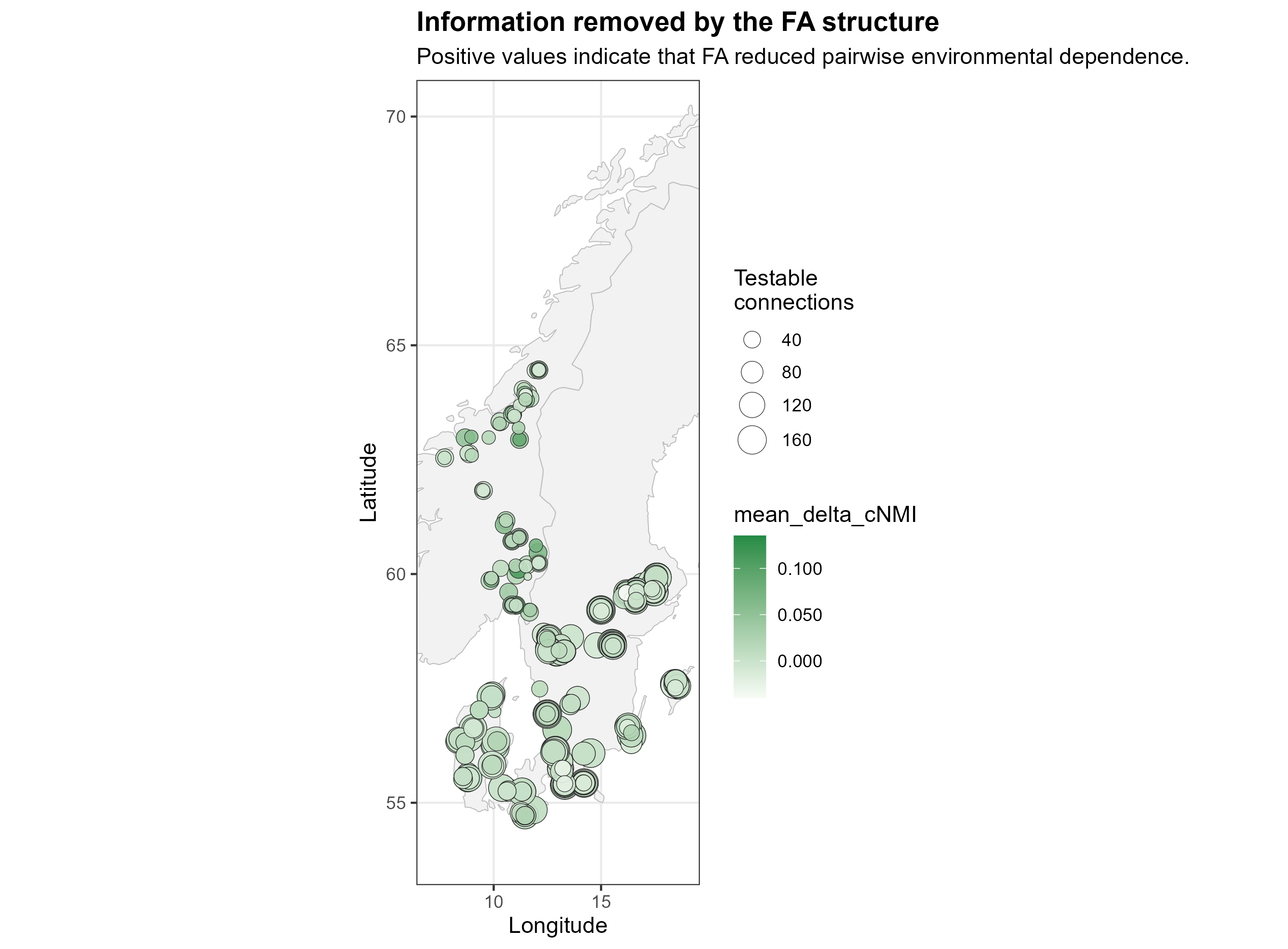
Information removed by FA for an environment pair:
\[ \Delta cNMI_{e_1 e_2} = cNMI^{pre}_{e_1 e_2} - cNMI^{post}_{e_1 e_2} \qquad (\text{not a proportion of variance}). \]
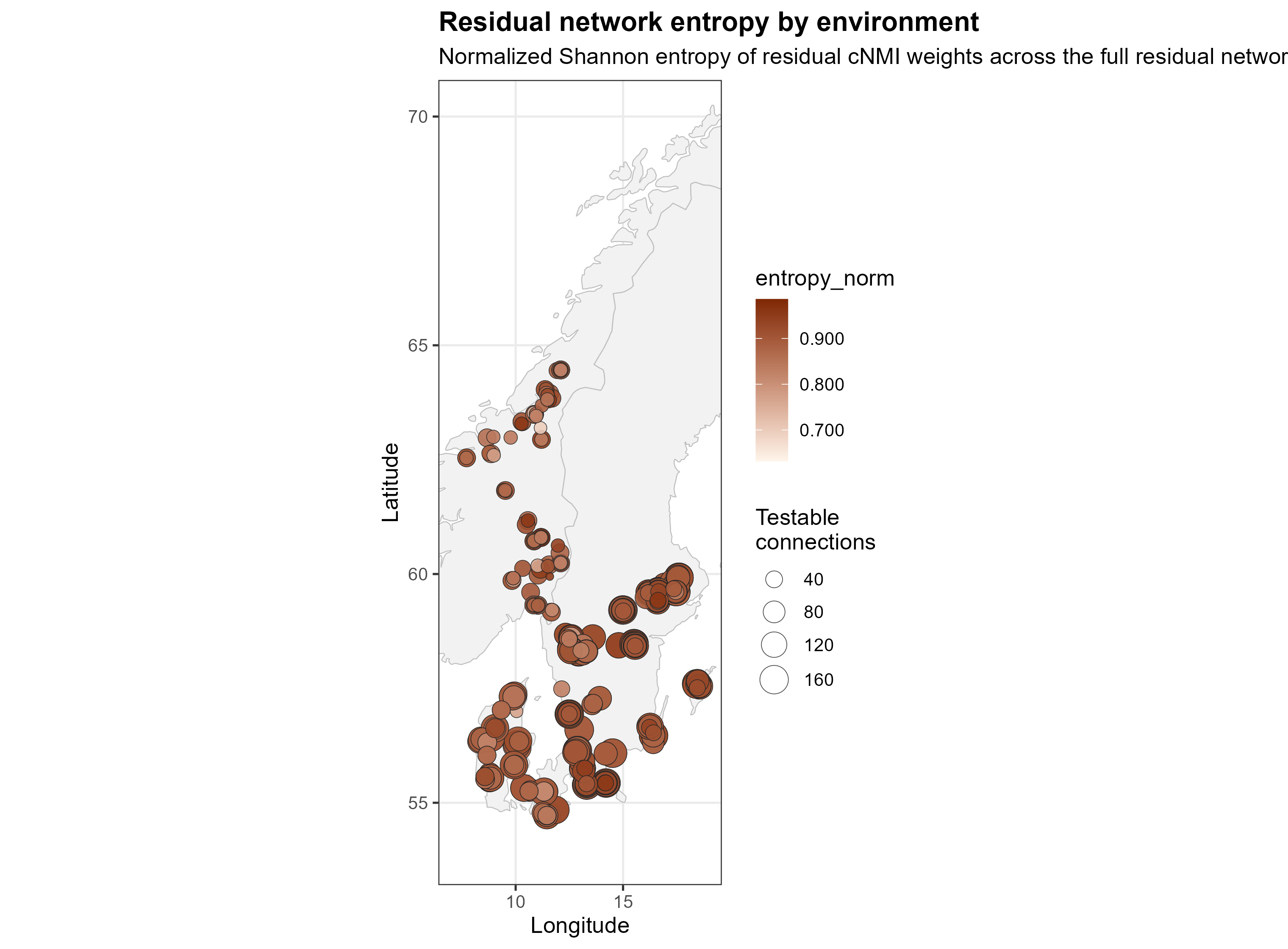
For environment \(e\), its positive residual links are normalized into a distribution, and Shannon entropy measures whether the dependence is concentrated in a few partners or diffuse:
\[ p_{ej} = \frac{cNMI_{ej}}{\sum_j cNMI_{ej}}, \qquad H_e = -\sum_j p_{ej}\log p_{ej}, \qquad H_e^{*} = \frac{H_e}{\log k_e}, \qquad \text{effective partners} = e^{H_e}. \]
From the equations to R
Condensed excerpts of the repository scripts (comments translated). Hover over the numbers to link each line to its equation.
mi_fast <- function(x, y) {
tab <- table(x, y)
pxy <- tab / sum(tab)
px <- rowSums(pxy); py <- colSums(pxy)
expected <- outer(px, py)
ok <- pxy > 0
sum(pxy[ok] * log(pxy[ok] / expected[ok]))
}- 1
- Joint \(p(x,y)\) and marginals \(p(x)\), \(p(y)\) from the contingency table.
- 2
- \(p(x)\,p(y)\): what the joint distribution would be under independence.
- 3
- Skip empty cells (\(0 \log 0 = 0\)).
- 4
- \(MI = \sum p(x,y)\log\frac{p(x,y)}{p(x)p(y)}\).
validate_pair_mi <- function(env1, env2, M, B = 199, nbins = 3) {
x <- M[, env1]; y <- M[, env2]
ok <- complete.cases(x, y); x <- x[ok]; y <- y[ok]
xd <- discretize_pair(x, nbins); yd <- discretize_pair(y, nbins)
MI_obs <- mi_fast(xd, yd)
NMI_obs <- MI_obs / sqrt(entropy_fast(xd) * entropy_fast(yd))
MI_perm <- replicate(B, mi_fast(xd, sample(yd)))
MI_corrected <- max(0, MI_obs - mean(MI_perm))
# ... NMI, empirical p-value and diagnostics follow
}- 1
- Only cultivars tested in both environments.
- 2
- Equal-frequency discretization into 3 classes.
- 3
- \(NMI = MI / \sqrt{H(X)H(Y)}\).
- 4
- Null distribution: permuting \(Y\) keeps \(n\), class frequencies and marginal entropies.
- 5
- \(cNMI = \max\{0,\ NMI_{obs} - \overline{NMI}_{perm}\}\).
fit_fa_order <- function(d, k, label) {
fa_terms <- paste0("FA", seq_len(k))
random_term <- paste0("(0 + ", paste(fa_terms, collapse = " + "),
" || Environment)")
form <- as.formula(paste("z_FA ~ 0 + variety +", random_term))
lme4::lmer(form, data = d, REML = TRUE, control = LMER_CONTROL)
}- 1
-
Columns
FA1..FAkhold the cultivar loadings \(\lambda_{gh}\) from the SVD. - 2
-
||sets zero covariance between latent factors, a natural identification after the orthogonal SVD basis;Environmentgroups the random scores \(w_{eh}\). - 3
-
varietyis fixed: \(\alpha_g\). - 4
- REML fit; FA(1)–FA(3) are then compared by AIC, BIC, convergence and residual variance.
compute_shannon_entropy <- function(w) {
w <- w[is.finite(w) & w > 0]
p <- w / sum(w)
h <- -sum(p * log(p))
k <- length(p)
tibble(entropy_shannon = h,
entropy_norm = if (k > 1) h / log(k) else 0,
effective_partners = exp(h),
concentration_hhi = sum(p^2))
}- 1
- Positive residual cNMI links of one environment.
- 2
- \(p_{ej}\): share of each partner.
- 3
- \(H_e = -\sum p_{ej}\log p_{ej}\).
- 4
- \(H_e^{*} = H_e / \log k_e\): 1 means evenly spread, near 0 means concentrated.
- 5
- \(e^{H_e}\): how many “equally strong” partners the environment effectively has.
Results
- FA(3) had the lowest BIC in both subsets (FA10 and FA15). Residual variance fell from 0.617 (FA1) to 0.535 (FA3), and the three factors explained 38.8%, 31.2% and 30.0% of the common factor variance.
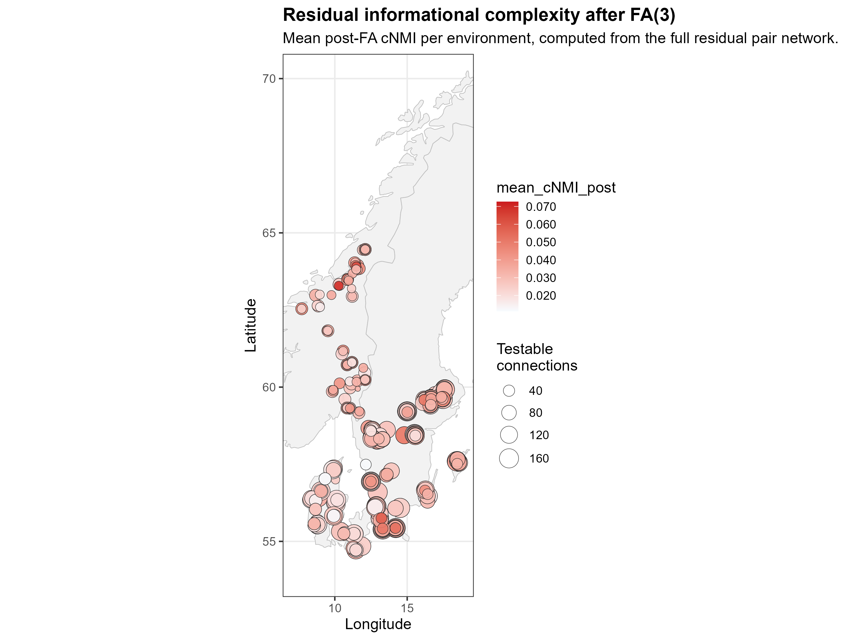
- Across 23,691 environment pairs, mean cNMI was 0.0300 before FA and 0.0271 after: 41.9% of pairs kept positive residual information.
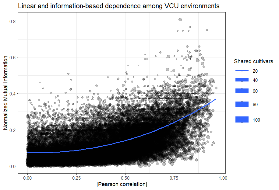
- Residual cNMI correlated only 0.345 with absolute Pearson correlation: information and correlation see different things.
- In the 200 preselected pairs, median residual NMI was 0.31 vs 0.09 under the matched linear null (98.5% with p ≤ 0.05). Because these pairs were preselected, this is not a prevalence over all pairs.
- Norway had the highest residual information and Sweden the most diffuse (highest-entropy) dependence.
ImportantAn honest negative result, kept on purpose
In Stage II, MI carried predictive signal but did not beat Pearson correlation as a global weight for predicting missing cultivar × environment cells. That is why MI is used here as a structural diagnostic, not as a universal replacement for correlation.
Open-science practices
Raw data come from the open Nordic MET dataset (Aasen et al., 2026; DataverseNO, DOI 10.18710/IZ3EFE, CC BY 4.0), with an MD5 checksum to prove the file is unchanged. The repository includes CITATION.cff, Zenodo and CodeMeta metadata, a GitHub Actions validation workflow, a data dictionary, provenance notes and a one-command run (Rscript scripts/run_all.R).
Skills shown: multi-environment trial analysis, factor-analytic mixed models, permutation tests, matrix completion, information theory, spatial visualization, research software engineering.